Page 43 - Demo

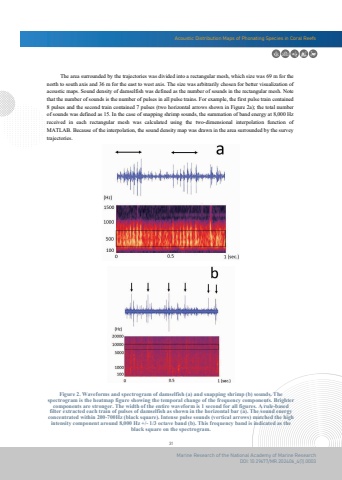
Acoustic Distribution Maps of Phonating Species in Coral Reefs31Marine Research of the National Academy of Marine ResearchDOI: 10.29677/MR.202406_4(1).0003 The area surrounded by the trajectories was divided into a rectangular mesh, which size was 69 m for the north to south axis and 36 m for the east to west axis. The size was arbitrarily chosen for better visualization of acoustic maps. Sound density of damselfish was defined as the number of sounds in the rectangular mesh. Note that the number of sounds is the number of pulses in all pulse trains. For example, the first pulse train contained 8 pulses and the second train contained 7 pulses (two horizontal arrows shown in Figure 2a); the total numberof sounds was defined as 15. In the case of snapping shrimp sounds, the summation of band energy at 8,000 Hz received in each rectangular mesh was calculated using the two-dimensional interpolation function ofMATLAB. Because of the interpolation, the sound density map was drawn in the area surrounded by the survey trajectories.Figure 2. Waveforms and spectrogram of damselfish (a) and snapping shrimp (b) sounds. Thespectrogram is the heatmap figure showing the temporal change of the frequency components. Brightercomponents are stronger. The width of the entire waveform is 1 second for all figures. A rule-basedfilter extracted each train of pulses of damselfish as shown in the horizontal bar (a). The sound energyconcentrated within 200-700Hz (black square). Intense pulse sounds (vertical arrows) matched the highintensity component around 8,000 Hz +/- 1/3 octave band (b). This frequency band is indicated as theblack square on the spectrogram.