Page 3 - 風機運維之結構振動與診斷

結構振動特性研究(1)

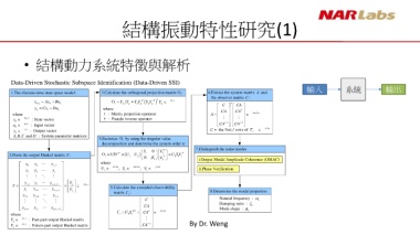
• 結構動力系統特徵與解析

Data-Driven Stochastic Subspace Identification (Data-Driven SSI)
輸入 系統 輸出

A
1.The discrete-time state space model: 3.Calculate the orthogonal projection matrix : 6.Extract the system matrix and
i
the observer matrix :
C
†

x k 1  Ax  k Bu k   Y Y  Y Y p T Y Y T  Y  li j C   CA 
f
p p
p
i
f
p
†
y  Cx  Du where 
k k k  CA   CA 2 
where / : Matrix projection operator A       2n 2n
x  2n 1 : State vector † : Pseudo inverse operator    
k  i 2   i 1 
u  m 1 : Input vector  CA   CA 
k
y  l 1 : Output vector C  the first rows of l  i  l 2n
k
A , , and : System parameter matricesB C D

4.Factorize by using the singular value
i
decomposition and determine the system order n:
 S 1 0  V   1 T T 7.Distinguish the noise modes
T
2.Form the output Hankel matrix : Y   USV  U 1 U 2    T    U S V
1 1 1
i
 0 S 2   V 2  i.Output Modal Amplitude Coherence (OMAC)
 y 0 y 1 y j 1  where
  U  li 2n , S  2n 2n , V  j 2n ii.Phase Verification
 y 1 y 2 y j  1 1 1
 
 y y y   Y 
Y   i 1 i i j  2    p   2li j
 y y y   Y 5.Calculate the extended observability
 i i 1 i j  1  f    matrix : 8.Determine the modal properties

 y i 1 y i 2 y i j  i
   C  Natural frequency :  k
   CA  Damping ratio :  k
 y 2 1i y 2i y 2i j    2  1/2  2  li 2n Mode shape :  k
where   U S    CA   
1 1
i
Y  li j : Past-part output Hankel matrix  
p
Y  li j : Future-part output Hankel matrix   CA  i 1  By Dr. Weng
f